Simply put, the chi square distribution is the distribution of the chi square statistic. So, when you want to understand more about the chi square distribution, you need to first determine the chi square statistic and only then find the probability associated with this statistic.

So, let’s get started.
As we mentioned above, the first step that you need to take to determine the chi square distribution is to determine the chi square statistic. So, let’s say that you run a statistical experiment where you’ll select a sample from a normal population – noted as “n”, and that has a standard deviation, noted as “σ”.
Take a look at the chi square reference table.
Along with our research and study, we discover that the standard deviation in the sample we are observing is “s”.
According to all these data, we can define the chi square statistic using the following formula:

However, what we want to determine is the chi square distribution which is simply the distribution of the chi square statistic. In order to do so, you will need to use the probability density function:
![]()
where,
Y0 – is a constant and it depends on the number of degrees of freedom
X2 – is the chi square statistic
v – V = n – 1 and is the number of degrees of freedom
e – is a constant and is equal to approximately 2.71828 (the base of the natural logarithm system)
While you may be a bit confused with the formula, you don’t need to worry since the graphical representation tends to help to determine everything you want to know.
Discover how to read values on a chi square table.
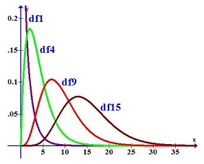
Let’s take a look at the graphical representation of the chi square distribution considering different samples of data.
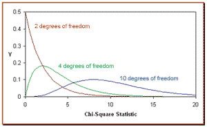
In this chart, you can see different curves with different colors:
– the red curve represents the chi square distribution when the samples of the population are 3. In this case, the number of degrees of freedom is 2 ( n – 1 = 3 – 1 = 2 ).
– the green curve represents the chi square distribution when the samples of the population are 5. In this case, the number of degrees of freedom is 4 ( n – 1 = 5 – 1 = 4 ).
– the blue curve represents the chi square distribution when the samples of the population are 11. In this case, the number of degrees of freedom is 10 ( n – 1 = 11 – 1 = 10 ).
Chi Square Distribution Properties:
- When you have degrees of freedom that are equal or higher than 2, the maximum value for Y will occur when X^2 = v-2.
- The mean of the distribution is always equal to the number of degrees of freedom.
- When you increase the degrees of freedom, you will see the chi square curve approaching the normal distribution.
- The variance is always equal to the number of degrees of freedom multiplied by 2.
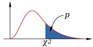
The Cumulative Probability
One of the things that you need to know is that the area under the curve of the chi square distribution and above 0 is a cumulative probability that s associated with the chi square value.