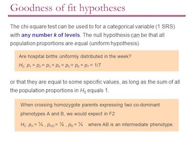
When you are learning statistics, it is natural that you already heard about the chi square goodness of fit test. According to our findings, many students struggle when they need to run this kind of test. So, today, we decided to give you a practical example of the chi square goodness of fit test.
Discover everything you need to know about the chi square test.
Let’s assume that you got a sample of Toronto women that were subjected to abuse by their partners.
Age – Number in Sample – Percent In Census
20-24 – 103 – 18
25-34 – 216 – 50
35-44 – 171 – 32
Total: 490 – 100
So, you want to run the chi square goodness of fit test based on the data of the previous table to determine whether the sample provides a good match to the known age distribution of Toronto women. Let’s say that you want to use the 0.05 significance level.

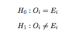
So, the first thing that you will need to do is to write down both the null hypothesis as well as the alternative hypothesis. In this case, the null hypothesis would be that the age distribution of women in the sample closely matches the age distribution of all women in Toronto. The alternative hypothesis would be that the age distribution of the women in the sample doesn’t match the age distribution of all Toronto women:
H0: The age distribution of respondents in the sample is the same as the age distribution of Toronto women, based on the Census.
H1: The age distribution of respondents in the sample differs from the age distribution of women in the Census.
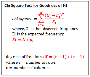
The frequencies of occurrence of women in each age group are given in the middle column of the table we displayed above. These are the observed values Oi, and there are k = 3 categories into which the data has been grouped so that i = 1, 2, 3.
Make sure to use our chi square calculator.
Imagine that the age distribution of women in the sample conforms exactly with the age distribution of all Toronto women as determined from the Census. Then, the expected values for each category, Ei, could be determined. With these observed and expected numbers of cases, the hypotheses can be written as follows:
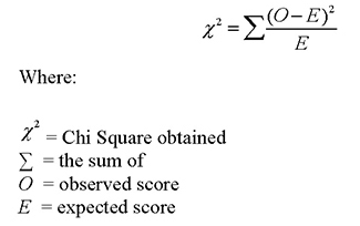
For these hypotheses, the test statistic is:
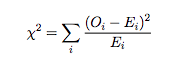
It’s important to notice that the chi square test should always be conducted using the actual number of cases, rather than the percentages. These actual numbers for the observed cases, Oi, are given as the frequencies in the middle column of the same table. The sum of this column is the sample size of n = 490.
So, the expected number of cases for each category is obtained by taking the total of 490 cases, and determining how many of these cases there would be in each category if the null hypothesis were to be exactly true. The percentages in the last column of the table are used to obtain these. Let the 20-24 age group be category i = 1. The 20-24 age group contains 18% of all the women, and if the null hypothesis were to be exactly correct, there would be 18% of the 490 cases in category 1. This is:
![]()
For the second category 25-34, there would be 50% of the total number of cases, so that:
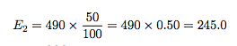
cases. Finally, there would be:
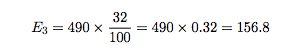
cases in the third category, ages 35-44.
You can use our simple chi square calculator to determine the chi square value.
Replacing in the formula:
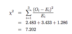
The next step is to decide whether this is a large or a small χ 2 value.
As we mentioned, the level of significance requested is the α = 0.05 level. The number of degrees of freedom is the number of categories minus one. There are k = 3 categories. So:
d = k −1 = 3−1 = 2 degrees of freedom.
By using the table, you can then see that the critical value is χ 2 = 5.991. This means that there is exactly 0.05 of the area under the curve to the right of χ 2 = 5.991.
Make sure to confirm your result with our calculator.
A chi square value larger than this leads to rejection of the null hypothesis, and a chi square value from the data which is smaller than 5.991 means that the null hypothesis cannot be rejected. The data yields a value for the chi squared statistic of 7.202 and this exceeds 5.991. Since 7.202 > 5.991 the null hypothesis can be rejected, and the research hypothesis accepted at the 0.05 level of significance.